Deep Learning from Scratch (Part 9) – Inside a Neural Network

So far in this series, we have worked with machine learning models that take inputs and produce predictions.

A neural network does the same thing.

The main difference is what happens between the input and the prediction.

Instead of using a single equation, a neural network passes the information through a collection of small computational units called artificial neurons. Each neuron performs a simple calculation. When many of them work together, the network can learn much more complicated patterns.

Let’s open the black box and look inside.

The Basic Structure

A neural network usually has three types of layers:

• an input layer,
• one or more hidden layers,
• and an output layer.

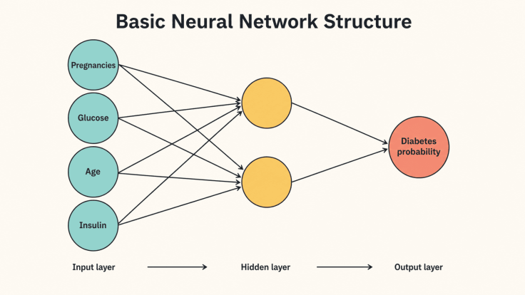
The input layer receives the values from our dataset.

The hidden layers process those values. They are called hidden because we do not directly observe what they produce as the final answer.

The output layer produces the prediction.

For example, imagine that we want to predict whether a patient has diabetes. Our inputs might include the patient’s glucose level, age, insulin level, and number of pregnancies.

The output could be a single number representing the predicted probability of diabetes.

The values move from the input layer to the hidden layer and then to the output layer.

This forward movement is called forward propagation.

But before following the values through the whole network, we need to understand what happens inside a single neuron.

What Does an Artificial Neuron Do?

An artificial neuron is the smallest computational unit in a neural network.

Despite the name, its calculation is quite simple:

1. Receive some inputs.
2. Multiply each input by a weight.
3. Add the results.
4. Add a bias.
5. Pass the total through an activation function.

That is the entire job of one neuron.

Let’s look at each part.

Inputs

Inputs are the values entering the neuron.

In the first hidden layer, they usually come from the dataset. In later layers, they come from neurons in the previous layer.

This means that one neuron’s output can become another neuron’s input.

Weights

Every input has a weight.

A weight controls how strongly that input affects the neuron. A large positive weight can push the result upward. A negative weight can pull it downward. A weight close to zero makes the input less influential.

Learning in a neural network is largely the process of finding useful values for these weights.

Bias

The bias is another value added to the calculation.

It gives the neuron some flexibility. Without a bias, the neuron is more restricted because its behavior depends entirely on the weighted inputs.

The bias is not chosen once and forgotten. Like the weights, it is adjusted while the network learns.

The Weighted Sum

Suppose a neuron receives three inputs:

$x_1 = 12,\qquad x_2 = 15,\qquad x_3 = 20$

For simplicity, let each weight be (0.1), and let the bias be (1).

The neuron first calculates:

$z = (12 \times 0.1) + (15 \times 0.1) + (20 \times 0.1) + 1$

So:

$z = 5.7$

This value is usually called (z), the weighted sum, or the net input.

At this point, the neuron has combined several pieces of information into one number.

It then sends (z) to an activation function.

If we use the sigmoid function in this example, the output is approximately:

$a = 0.9966$

The letter (a) stands for the neuron’s activation.

For now, the important relationship is:

$\text{inputs} \rightarrow z \rightarrow a$

First, the neuron calculates the weighted sum (z). Then the activation function transforms it into (a).

We will examine activation functions properly in the next post. Here, we only need to know that they transform the weighted sum before passing information forward.

From One Neuron to a Network

Now let’s return to the diabetes example.

We have four input values for one patient:

Feature	Value
Pregnancies	6
Glucose	148
Age	50
Insulin	0

We will send these values into a hidden layer containing two neurons.

The number of hidden layers and neurons is something we choose when designing the network. These choices are called hyperparameters. For this example, two neurons are enough to see how the calculation works.

Every input is connected to every neuron in the hidden layer.

Each connection has its own weight, and each hidden neuron has its own bias.

The numbers below are only illustrative. In a real network, the useful weight and bias values would be found during training.

Calculating the First Hidden Neuron

For the first hidden neuron, suppose the weights are:

$0.1,\quad 0.3,\quad 0.5,\quad 0.7$

and the bias is:

$b_1 = 0.1$

Its weighted sum is:

$z_1 = (6 \times 0.1) + (148 \times 0.3) + (50 \times 0.5) + (0 \times 0.7) + 0.1$
$z_1 = 70.1$

After applying the sigmoid function, the activation is approximately:

$a_1 \approx 1.0$

Calculating the Second Hidden Neuron

For the second neuron, suppose the weights are:

$0.2,\quad 0.4,\quad 0.6,\quad 0.8$

and the bias is:

$b_2 = 0.2$

Its weighted sum is:

$z_2 = (6 \times 0.2) + (148 \times 0.4) + (50 \times 0.6) + (0 \times 0.8) + 0.2$
$z_2 = 90.6$

After applying sigmoid:

$a_2 \approx 1.0$

We now have two activations:

$a_1 \approx 1.0,\qquad a_2 \approx 1.0$

The original four inputs have been transformed into two new values.

These two activations become the inputs of the output neuron.

Producing the Final Prediction

Suppose the weights leading to the output neuron are (0.3) and (0.4), and its bias is (0.5).

The output neuron calculates:

$z_{\text{out}} = (a_1 \times 0.3) + (a_2 \times 0.4) + 0.5$

Using our activation values:

$z_{\text{out}} = (1.0 \times 0.3) + (1.0 \times 0.4) + 0.5$
$z_{\text{out}} = 1.2$

After applying sigmoid one more time:

$\hat{y} \approx 0.77$

In this binary classification example, we can interpret the result as a predicted probability of approximately 77% for the positive class.

And that is one complete forward pass.

The information started as four patient measurements. It moved through two hidden neurons and ended as one prediction.

What Has the Network Learned?

Nothing yet.

We used example weights and biases to make a prediction, but we do not know whether that prediction is correct.

The network still needs to compare its prediction with the actual answer, measure the error, and adjust its weights and biases.

That adjustment process is how the network learns.

For now, the important idea is simpler:

A neural network is not one mysterious calculation. It is a collection of small calculations connected to one another.

Each neuron takes inputs, applies weights and a bias, and produces an activation. Those activations move forward until the network produces a prediction.

In the next post, we will slow down at the step we briefly passed over here and look at activation functions.